EMD Basic

Introduction

Empirical Mode Decomposition (EMD) is a non-linear and non-stationary data analysis technique with the ability to extract AM-FM components, called Intrinsic Mode Functions (IMFs), of the signal, in the time domain itself (Huang et al., 1998).

EMD is similar to Fourier Transform (FT). FT assumes our signal is periodic and it’s basic components are various simple sine waves. And FT makes our signal from time domain to frequency domain. The different with EMD is the output remains in the time spectrum and EMD dose not assume our signal is periodic and it’s not based on simple sine wave instead, it’s Intrinsic Mode Function (IMF). EMD is really based on the dataset, doesn’t have an assumption about the data (That why it’s called Empirical).

Detail

Overview

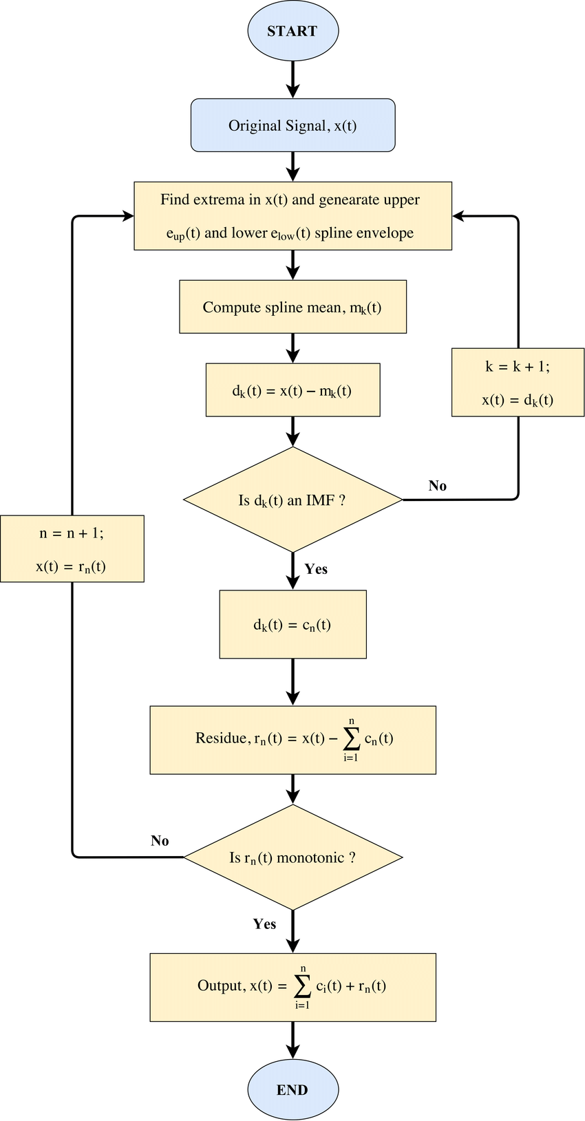
Flow Chart

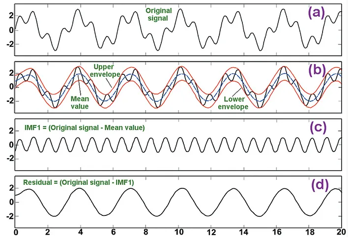
Step by Step

Input $x(t)$,

1. Identify all extrema of $x(t)$
2.  Create an envelope of minima and maxima from the array of minima and maxima.
   • Interpolate the value of minima and maxima to create an envelope of minima and maxima using a cubic spline.
   • maxima envelope: $e_{\text{max}}(t)$
   • minima envelope: $e_{\text{min}}(t)$
3. Compute the mean from the envelope of minima and maxima $m(t)=\frac{e_{\text{max}}(t)+e_{\text{min}}(t)}{2}$
4. Extract the detail $c(t)=x(t)-m(t)$
5. Iterate 1-4 with $x(t)\leftarrow c(t)$ until $c(t)$ is zero-mean
   • or some stopping criteria
   • The resulting $c(t)$ is the intrinsic mode function (IMF)
6. Iterate 1-5 on the residue $m(t)=x(t)-\sum c_i(t)$
   • Until some stopping criteria
     • Peak Frequency is low
     • Residuum signal is just a constant, monotonic, or just have 1 extremum

Hilbert Spectral Analysis (HSA)

Instantaneous Frequency

To see:

Instantaneous Frequency⭐

HSA after EMD

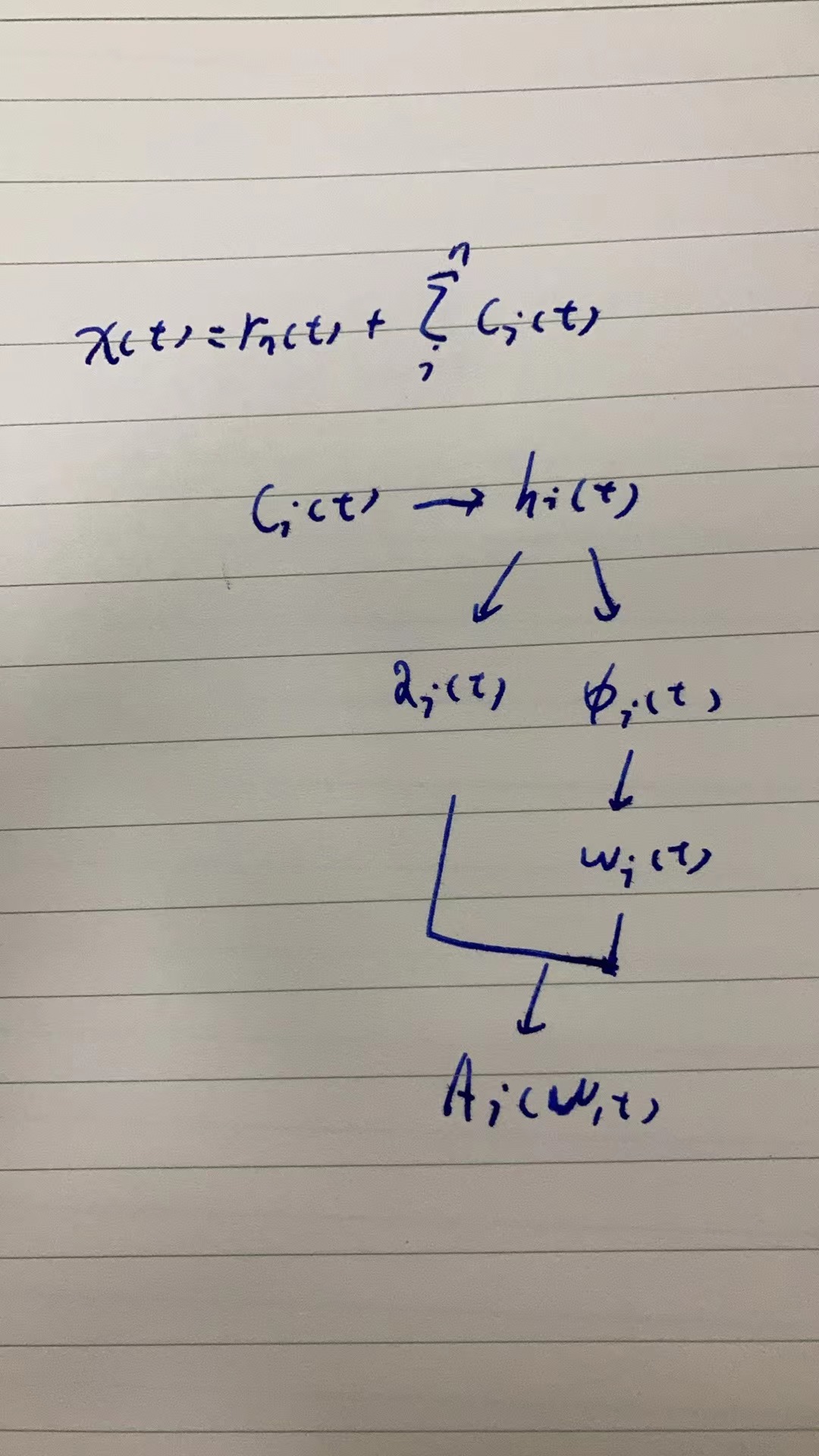
得到这些IMF之后，我们的信号$x(t)$可以表达为，

$$x(t)=r_n(t)+\sum _i^n{c}_i(t)$$

进而我们会通过这个$x(t)$的表达去得到时频分析图；如上图所示，得到这个时频分析图的过程中，不会用到最后的剩余部分$r_n(t)$，因为它要么是单调函数，要么是常数。尽管希尔伯特变换可以将单调趋势视为较长振荡的一部分，但残余趋势中涉及的能量可能会非常强大。考虑到较长趋势的不确定性，并且为了其他低能量和高频分量中包含的信息的利益，最终的非 IMF 分量应被排除。然而，如果物理考虑证明其包含是合理的，则可以将其包含在内。这是一个Tradeoff。

然后，通过对IMF分量做Hilbert Transform构建analytic signal，

$$h_i(t)=c_i(t)\times \frac{1}{\pi t}=\frac{1}{\pi }\text{p.v.}{\int }_{-\infty }^{\infty }\frac{c_i(\tau )}{t-\tau }d\tau$$

构建出来的解析信号为，

$$A_i(t)=c_i(t)+i{H}_i(t)={\alpha }_i(t)e^{i{\theta }_i(t)}$$

进而得到瞬时幅值和瞬时相位，进而通过瞬时相位得到瞬时频率，

$${\alpha }_i(t)=\sqrt{c_i(t{)}^2+h_i(t{)}^2},\theta (t)=\arctan (\frac{h_i(t)}{c_i(t)}),\omega =\frac{d{\theta }_i(t)}{t}$$

进而，最后我们可以进行HSA，即

$$\text{Plot}{H}_i(\omega ,t)=\{\begin{array}{ll}{\alpha }_i(t),& \omega ={\omega }_i(t)\\ 0,& \text{otherwise}\end{array}H(\omega ,t)=\sum _{i=1}^n{H}_i(\omega ,t)$$

Demo code

import numpy as np
import numpy as np
 
def EMD(signal, max_imf = 10, tolerance = 0.01):
    
    def __extrema(signal):
        
        max_peaks = []
        min_peaks = []
        
        for i in range(1, len(signal) - 1):
            if signal[i] > signal[i-1] and signal[i] > signal[i+1]:
                max_peaks.append(i)
            if signal[i] < signal[i-1] and signal[i] < signal[i+1]:
                min_peaks.append(i)
                
        return max_peaks, min_peaks
    
    
    def __mean_env(signal):
        
        max_peaks, min_peaks = __extrema(signal)
        
        max_env = np.interp(range(len(signal)), max_peaks, [signal[i] for i in max_peaks])
        min_env = np.interp(range(len(signal)), min_peaks, [signal[i] for i in min_peaks])
        
        return (max_env + min_env) / 2
    
    def __IMF(signal):
        
        resdiual = signal
        
        while True:
        
            imf = signal - __mean_env(resdiual)
            resdiual = signal - imf
            
            if np.mean(imf) < tolerance:
                break
        
        return imf, resdiual
    
    # standardize the signal
    mean = np.mean(signal)
    std = np.std(signal)
    
    signal = (signal - mean) / std
    
    imfs = []
    
    while True:
        
        imf, residual = __IMF(signal)
        
        imfs.append(imf)
        
        max_peaks, min_peaks = __extrema(residual)
        
        if len(max_peaks) < 2 or len(min_peaks) < 2:
            break
        
        if np.abs(np.std(residual)) < tolerance or max_imf == 0:
            break
        
        signal = residual
        max_imf -= 1
        
    imfs = [imf * std + mean for imf in imfs]
    residual = residual * std + mean
        
    return imfs, residual

Download Step by Step Slides

Slides

Reference

• Huang, Norden E., et al. “The Empirical Mode Decomposition and the Hilbert Spectrum for Nonlinear and Non-Stationary Time Series Analysis.” Proceedings of the Royal Society of London. Series A: Mathematical, Physical and Engineering Sciences, vol. 454, no. 1971, Mar. 1998, pp. 903–95. DOI.org (Crossref), https://doi.org/10.1098/rspa.1998.0193.
• https://www.youtube.com/watch?v=K-LhNvr-CSk
• https://towardsdatascience.com/decomposing-signal-using-empirical-mode-decomposition-algorithm-explanation-for-dummy-93a93304c541⭐
• https://en.wikipedia.org/wiki/Hilbert_spectrum
• https://www.youtube.com/watch?v=BLUL8i0KzKg